Alternate Row Shading

Alternate Row Shading – an easy way to enhance readability, attractiveness, and style

Sometimes, the simplest edits can greatly enhance your presentation. For example, refer to the 2 exhibits below.

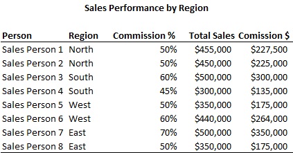
When presenting a sizeable list of items with various columns, the reader may struggle at tracking all the information you are trying to convey. Adding alternate row shading helps the user track a specific row of data with ease.

Adding alternate row shading is quite easy. Just highlight the region where you want to add the shading, then go to Format > Conditional Formatting. Then choose the option to write in your own formula. Type in the following:

=mod(row(),2)=0

Then choose a fill color for your formatting. The exact steps vary between the different versions of Excel, but the general idea remains the same.

Let’s break down this formula. The “Mod()” function takes a number, divides it by the second number, and returns the remainder. The “Row()” function returns the current row. So what the formula does, is that it takes the current row, divides it by 2, and gives the remainder. The remainder will alternate between 1 and 0 depending on your row, since whenever you divide something by 2, the remainder can only be 1 or 0. If it is a 0, then perform the formatting, if it is 1, then do nothing. Keep in mind that you can edit the formatting however you desire. It does not have to be a fill, instead it can be a change in text color, font, borders, etc.

Suppose you want to shade 2 lines at a time, how would you do that? Use the following formula:

=mod(row(),4)>1

Then choose a fill color for your formatting. This formula takes the current row, divides it by 4. The remainders can either be 0, 1, 2, or 3. If it is greater than 1 (2 or 3), then shade it, else (0 or 1) leave it alone. As a result, 2 rows are shaded at a time.

If you want to shade every 4^th row, then use:

=mod(row(),4)>2

Then choose the formatting you want. You may need to adjust the number of rows before your exhibit begins to get it to shade the 4^th row. In other words, you may need to paste or delete rows around your exhibit to adjust the where the shading occurs.

To see these exhibits on a spreadsheet, please download it here.

Formatting - call me superficial, but aesthetics do matter (part 1)

Formatting – call me superficial, but aesthetics do matter (part 1)

Whenever I am working on a spreadsheet, I always like to be thoughtful about the viewer and the medium.  For example, if I know that the viewer will be a client paying extravagant fees for my work, I want my work to be stylish, clean, elegant, and near perfect.  In this case, my work will most likely be pasted into a deck, so design and simplicity is more important than functionality and flexibility.  On the contrary, if I know that other analysts will be editing and tinkering with my spreadsheet, I want to focus on functionality, flexibility, and ease of manipulation.

Suppose you want to present the data below to a client in a deck.

Clearly, the information isn’t presented in a very attractive manner.  The numbers should be formatted, gridlines removed, titles bolded, headings for numerical columns right aligned, borders drawn in, etc.  Below are a few ways to enhance the look and feel.

A minimalist approach, used for those that prefer simplicity:

A trendy, modern approach, used for those that like to add some style to their data.  Notice the use of alternate row shading to make it easier for the user to differentiate between rows.

A boxier, conventional approach, used for those who prefer a more conservative look.

As you can see, there are many things you can do to add style and creativity in presenting your findings.  Of course, there’s no right or wrong approach; the important thing is to be thoughtful of the context and your purpose.  If a certain column is more important than the rest, then go ahead and box it, bold it, give it a different color, etc.  If something looks ugly, then think about how to make it look better.  If your company uses a standard color scheme, then use those colors.  There truly is an infinite number of possibilities in designing client-ready, value-added exhibits.

However, there are certain things that I like to do.  I generally don’t like to merge cells when centering words over multple cells, because I feel that it makes it more difficult to manipulate your exhibits later on.  Instead, I type in the word in the left most cell of the region that I want to center across, highlight the region, then choose “Center Across Selection” under Format Cells > Alignment (highlight region, CTRL + 1, Alignment tab).  I generally like to keep my titles short.  If they are too long, I use multiple rows.  I like to group headings together under 1 heading if they are related.  For example, I grouped “Projected Yearly Sales” and “R&D Expense” under “Financials”.  Columns should be as thin as possible so that the exhibit itself can be blown up on a deck.  I also like to remove gridlines on exhibits.  Gridlines are helpful when you are running calculations or modeling, but they are ugly.  Therefore, they should not be included in a client exhibit.

To see the exhibits that I built on a spreadsheet, please click here.

Why pivot tables rock

Why pivot tables rock, especially compared to arrays (but arrays are still awesome)

Do you ever run into situations where you have a large amount of data, and you need to perform some type of mathematical operation on a subset of your data?  For example, maybe you want to sum up all the sales within a certain region, find the average of sales for a certain manager, or find the sales value of the highest seller for each manager in the example below.

One method to do each of these calculations is to write an array.  However, I think that it is much quicker to use a pivot table.

To Find the Sales within a Certain Region

1. Pivot the data
2. Set the Report Filter (at the top) to be “Region”
3. Set values to be “Total Sales”
4. Right click on the data, choose Value Field Settings, then choose Sum.
5. Now you can adjust the region and see the sales for each region.

To Find the Average of Sales for a Certain Manager

1. Pivot the data
2. Set values to be “Total Sales”
3. Set row labels to be “Manager”
4. Right click on the data, choose Value Field Settings, then choose Average.
5. Now you can see the average sales for each manager.

To Find the Sales Value of the Highest Seller for each Manager

1. Pivot the data
2. Set values to be “Total Sales”
3. Set row labels to be “Manager”
4. Right click on the data, choose Value Field Settings, then choose Max
5. Now you can see the highest sales value for each manager.
6. If you want to see who the sales person is, add “Salesperson” to the Row Label. The pivot table will stack Manager and Salesperson together, and show you the sales for each salesperson.

Pivot tables are an extraordinarily powerful tool that lets the user slice and dice data very quickly.  Spend some time playing around with the pivot table by putting fields in different areas and stacking them on top of each other.  Also, experiment with changing the field settings around from Max to Sum to Min to Average, etc.  Trust me, this will pay huge dividends in the future.

Another thing to note about pivot tables is that they can aggregate similar lines of data together.  For example, if you have 2 rows of data for Joe, the pivot table will automatically sum up the sales for Joe if you run a pivot to view Salesperson and Total Sales.  In other words, the pivot table will automatically combine sales together if they are derived from the same source.  Joe will not show up as 2 separate lines in the pivot table, instead, he will show up as 1 line, but include the sum of both lines of data.  If you have a massive data set with many lines of data for the same salesperson, the pivot table will automatically sum up all those sales for you.

Below is an example of data with multiple entries for certain salespeople.

A pivot table can quickly summarize the data for you.

Then you can copy and paste this pivot table and reformat it to your liking.  Please click here to check out the sample spreadsheet associated with this post.

The beauty of copy and paste...

The beauty of copy and paste

Copying and pasting has saved me so much time on so many occasions.  Assuming you’ve already done something once, why repeat it again?  The more efficiently you can get something done, the more your time frees up for other tasks.  Most people are probably familiar with copying cells of data.  I will try to expand on that same concept by taking it to another level.

Copying entire rows and columns

Suppose you already have a complicated spreadsheet with working formulas, cell references, and various lookups.  See below.  Bill rates, hours, and cost for each contractor are broken up quarterly.  Quarterly Cost of contractor = quarterly bill rate * quarterly hours.  Then suppose you need to expand on that spreadsheet to accommodate quarter 3. 

Instead of inserting blank columns and rewriting the formulas, just copy and paste columns E, H, and J, one at a time.  To copy, highlight the entire column, copy, then paste as a new column. (CTRL + Space, CTRL + C, CTRL + SHIFT + “+”).  Then rename the newly created columns to reflect Q3 and update the data for Q3 Bill Rate and Q3 Hours.  The formulas for Q1 Cost and Q2 Cost should not be impacted by the copy and paste.  The formulas for Q3 Cost should already reflect Q3 Bill Rate * Q3 Hours.  When you added the new columns, since no cells were locked, Excel knows to shift over the formula for Q3 Cost.

Now suppose you want to add a new contractor to the list.  No need to start off with a blank row and rewrite all the formulas.  Just simply highlight one of the rows and re-paste it (SHIFT + Space, CTRL + C, CTRL + SHIFT + ”+”).  Now you should have a duplicate row.  Just replace the non-formulaic data in that duplicate row.  The costs should automatically update for that new person since all the formulas were kept intact.

Although this is a very simple example, it shows how much time you can save by just copying and pasting entire rows and columns, especially if you have a spreadsheet saturated with very similar formulas.

Copying Formatting

Sometimes, you may spend a lot of time formatting an exhibit to get it to look just right.  Then you realize that you have to do the same formatting to 10 other exhibits for consistency.  In that case, you can simply copy the formatting from the original exhibit over to the other exhibits.  If the exhibits are exactly the same size, then you can actually copy the entire exhibit, and paste formatting.  However, if the exhibits are different sizes, you may have to copy the formatting in several phases.

Suppose this is your original exhibit, and you want to transfer this formatting over to other exhibits.  Note that this exhibit contains conditional formatting to set the alternate row shading.

Suppose this is your unformatted exhibit.

What you can do is copy the formatting for the title, headings, and data.  First, select the row that you want to copy the formatting from then copy (CTRL + C).  Next, highlight the row where you want to transfer the formatting to.  Then paste special > formats (ALT, E, S, T, ENTER).  Using paste special > formats, you can quickly copy the look and feel of one exhibit to another exhibit.

Copying entire sheets

Suppose in the previous example, you needed the “Contractor Information” exhibit 12 times, but with a slight variation each time.  For example, maybe you need that same exhibit, but on a monthly basis from January to December.  And suppose you also need it on separate tabs so that other users can easily identify what exhibit they are looking at.  Just simply copy and paste the tab 10 times by right clicking on the tab, then “Move or Copy”, check “Create a Copy”, then OK.  In each copy, just make the tweaks necessary so that it reflects a specific month’s data.  The formatting should already be done.

Click here to download a spreadsheet with the above examples.

VLOOKUP and MATCH, the perfect couple

VLOOKUP and MATCH, the perfect couple…

A lot of you are probably familiar with VLOOKUPs, and a lot of you may even be familiar with the MATCH function, but did you know that you can combine them together and create magic?  Seriously, VLOOKUP + MATCH is like wine + cheese, Romeo + Juliet, or chips + salsa.

Suppose you have a spreadsheet with a lot of data.  Each order is unique and has the fields Plan, PM, Description, Cost, Rating, Value, and Quality associated with it.  For example:

Sheet1

Then suppose you want to transfer all this data to another sheet, but with only a subset of the above fields.  One way to do it is to set cell references.  But when you start cutting and pasting stuff, it will get confusing.  However, there is a way to use 1 formula to pull all the values that you need.  Here’s where the VLOOKUP + MATCH come in to play.  On a blank spread sheet (Sheet2), create the design for your output and choose the orders and fields that you want to display.

Sheet2

Then, you can write 1 formula to populate all the blank cells based on the order number and field title.  For example, in cell B2, write: =vlookup($A2,Sheet1!$A$1:$H$21,match(B$1,Sheet1!$A$1:$H$1,0),0)

Make sure that the arrays used in the VLOOKUP and MATCH function refer to the data sheet and not the sheet of your output.  This is important!

So, with the above formula, you can paste it into all the blank cells, and the formula will pull the data you need.  The VLOOKUP looks for the order number you specified, and the match function finds the specific field you are interested in.  Voila!  Same formula can be pasted repeatedly to pull different data points.  The locking that I have specified directs the formula to point at the relevant order number and field no matter where you paste the formula.

Keep in mind that you do not have to use the titles as your match range.  You can use a blank row above your titles and above your data to create a new match range.  E.g.

Data

Exhibit

In this case, you just set the MATCH range to the first row.  This allows you to set up your own naming convention for the MATCH function, so you’re not limited to the titles of your exhibit.  Just remember to reference your new MATCH range when you set the array for the MATCH function.

This VLOOKUP + MATCH concept is very powerful and useful for building exhibits, transferring data, or viewing data in a specific way.  It’s quick and efficient once you get the hang of it, and minimizes chances of error.

Here is a spreadsheet demonstrating my example.